Painless Chart Title Updates

I originally called this post “Dynamic Chart Titles in Excel”.

SEO-friendly, perhaps.  But it could have been catastrophic.

In weaponized form, that five-word combination could unleash a wave of drowsiness not seen in modern times.  Even in an 11-point font, it will cause you to blink for a second or two longer than normal.

Use with caution!

---

This post takes the tedious task of updating an Excel chart title and makes it less painful.  Typically, we send the same chart to the same people day after day after day after day…

You get the point.

To get us started, we’ll use a sample chart looking at my daily steps so far in August:

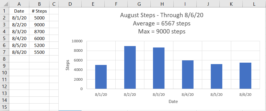
I want to track my daily step average and maximum step count for the month.  I also want the chart to update when I add more data.  The axis titles, “Steps” (y-axis) and “Date” (x-axis), stay the same but my chart title will change every day I add more information.

Doing this manually gets very old very quickly.

Any data moves require a micro-adjustment to the title.  No biggie until you realize that three minutes of daily tweaks costs you 12.5 hours of labor per year.

Egad!

No need to fret, however.  We can do it automatically.

Building the statistics

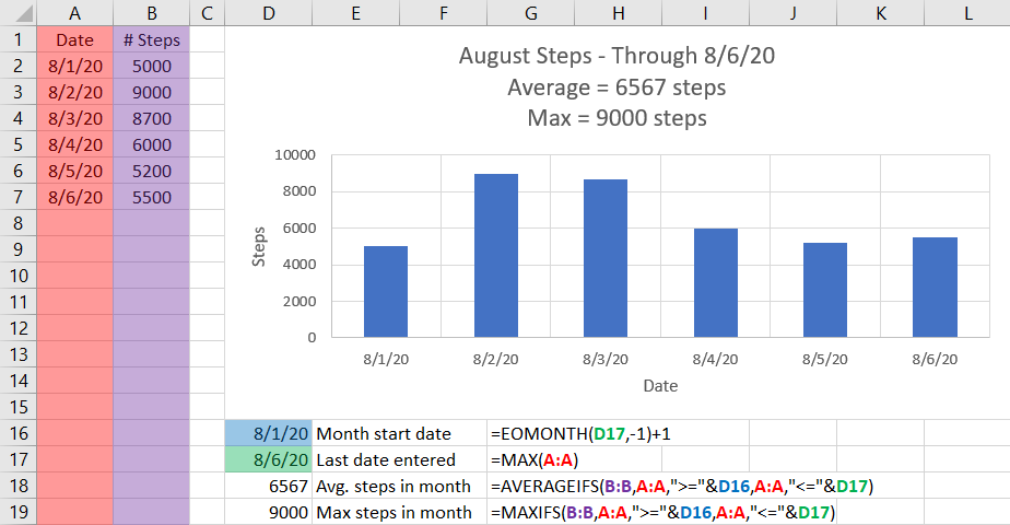
To start, we need to determine the month’s start date, last day of data entered, average steps for the month, and month’s maximum steps.

Briefly reviewing these formulae:

• Month start date:  EOMONTH(DATE, 0) returns the last day of DATE’s month (e.g. 7/5/2020 will yield 7/31/2020).  EOMONTH(DATE, -1) yields the last day of last month.  By adding 1, we get to the start of the current month!
• Last date entered:  Excel converts dates into the number of days after January 1, 1900 (or 1/1/1904 for some Mac users).  The largest number is the most recent date, hence the use of MAX().
• Avg. steps in month:  AVERAGEIFS() will average together all values in Column B with corresponding values, i.e. in the same row, that satisfy all conditions of the expression.  For example, B2 (value of 5000) will only be included if A2 (value of 8/1/20) is between the start of the month (D16 or 8/1/20) and the last date entered (D17 or 8/6/20). Since it satisfies all conditions, it is averaged in.
• Max. steps in month:  Similarly, MAXIFS() finds the largest value of Column B with corresponding dates between 8/1/20 and 8/6/20.

Building the title

Now, we can create a descriptive title that updates as we add more data by combining three separate lines:

1. August Steps – Through 8/6/20
2. Average = 6567 steps
3. Max = 9000 steps

The TEXT() function and ampersand “&” will come in handy.  Observe:

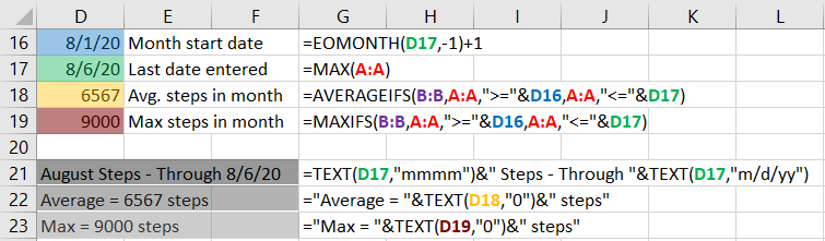
For the first title line (cell D21), we use TEXT() in two ways:

1. TEXT(D17,”mmmm”) converts “8/6/20” into month’s full name, i.e. “August”
2. TEXT(D17,”m/d/yy”) maintains the “m/d/yy” format in the formula result.  Without it, “44049” would appear in its place.

For more details on date formats used with the TEXT() function, check out this post.

Using “&” we can stitch together “August” with “ Steps – Through “ and “8/6/20” to complete the line.  Keep in mind that spaces are important in the connecting text.  Sans spaces,  “AugustSteps-Through8/6/20” borders on unreadable.

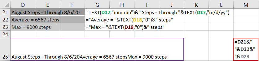
TEXT(D18,”0”) in cell D22 and TEXT(D19,”0”) in cell D23 keep each formula result as an integer for tidy reporting.  Without it, August’s average becomes 6566.66666666667 steps, an impressive (though ridiculous!) display of accuracy to within 10 picosteps.  “Average = “ and “Max = “ are tied with their corresponding statistic with “&” to complete each line.

To finish the title, we use “&” to combine these three lines (i.e. D21, D22,and D23) with line breaks (a.k.a. carriage returns) as shown in Cell M25 below (bordered in red).  Hold down the “Alt” key and then press “Enter” to insert the carriage return.  (Akin to “Shift+Return” used in several apps to insert a line without sending a message.)  This keeps the title clean with each statistic on a separate line.

Cell D25 (bordered in purple) is the output, though there is no evidence of carriage returns.  That’s ok.  We will see them in a second.

Our chart is now ready for the final step!

Automating the title

Select the chart title’s text box and click in the formula bar toward the top of the page.  Instead of typing in text, select cell D25 to reference our well-crafted title!

Voila!

Now comes the fun part.  When we enter the next day’s data, the title updates automatically!  Let’s try 10,000 steps for August 7th and see what happens:

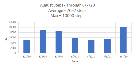
Bingo!

All our stats updated, including the new max steps for August, just by adding the data. A couple extra minutes of work should save you a ton time going ahead!

---

Thank you for reading! Feel free to add your comments below – what you liked or other Excel tricks worth learning about.

Shout out to Megan, Tyler, Joel, Eugene, Tom and colleagues at Compound Writing for your feedback!